Background and Motivation

The Paris Agreement of 2015 was an international standard laid out in order to reduce \(CO_2\) emissions. With the Paris Aggreement, national emmisions target and regulations sprung up in order to substantially reduce global greenhouse gas emmission to hold global temperature incear to well below 2 C.

With these new regulations, businesses were pressured to lower their emmissions. Thuse introducing carbon markets with the promise to turn \(CO_2\) into a commodity.

Carbon offsetting is a trading mechanism that allows entities such as governments, individuals, or businesses to compensate for their greenhouse gas emissions by supporting projects that reduce, avoid, or remove emissions elsewhere.

To Put it simply, carbon offsets involve an entity that emits greenhouse gases into the atmosphere paying for another entity to pollute less. For example, an airline in a developed country that wants to claim it is reducing its emissions can pay for a patch of rainforest to be protected in the Amazon.

The main research question I want to investigate is whether carbon credits are an effective way to measure carbon offset emissions. Each credit purportedly offsets a metric tonne of CO2 emissions, yet the Berkeley Carbon Trading Project reports that, “research performed by [them] and others has found that many, if not most, offset credits traded on the market today do not represent real emissions reductions.” [[^1]]

Goal

Combining the Voluntary Registry Offsets Data with another emissions data would be a helpful way to measure if carbon trading/offsets are accurate in measuring emissions.

Reserach Questions

The main research question is to see : Are climate credits being distrubuted evenly?

I will create three separate visualizations that same overall question: How has the Carbon Market grown over the years per country ? and are they keeping up with the global emission reduction goals

Each visualization below has been

Data

Link to (or otherwise prove the existence of) at least one data set that you plan to use for Assignment #4
- Berkeley Voluntary Registry Offsets Database: contains all carbon offset projects, credit issuances, and credit retirements listed globally by four major voluntary offset project registries
- Data on CO2 and Greenhouse emissions by Our World in Data
- Raster Data provided by Natural Earth

Code

##~~~~~~~~~~~~~~~~~~~~~~~~~~~~~~~~~~~~~~~~~~~~~~~~~~~~~~~~~~~~~~~~~~~~~~~~~~~~~~
##                           library setup                                 ----
##~~~~~~~~~~~~~~~~~~~~~~~~~~~~~~~~~~~~~~~~~~~~~~~~~~~~~~~~~~~~~~~~~~~~~~~~~~~~~~
library(tidyverse)
library(ggplot2)
library(ggExtra)
library(gghighlight)
library(janitor)
library(naniar)
library(RColorBrewer)
library(here)
library(forcats)

library(showtext)
font_add_google(name = "Merriweather", family = "merriweather")
font_add_google(name = "Karla", family = "karla")

font_add(family = "fa-6-brands",
         regular = here::here("fonts", "Font Awesome 6 Brands-Regular-400.otf"))
font_add(family = "fa-6-regular",
         regular = here::here("fonts", "Font Awesome 6 Free-Regular-400.otf")) 
font_add(family = "fa-6-solid",
         regular = here::here("fonts", "Font Awesome 6 Free-Solid-900.otf"))

font_add(family = "fa-brands",
         regular = here::here("fonts", "fa-brands-400.ttf"))
font_add(family = "fa-regular",
         regular = here::here("fonts", "fa-regular-400.ttf")) 
font_add(family = "fa-solid",
         regular = here::here("fonts", "fa-solid-900.ttf"))


library(raster)
library(countrycode)

library(ggtext)
library(ggrepel)
library(patchwork)
library(systemfonts)

library(fmsb)
library(stringr)

library(emojifont)
library(NatParksPalettes)

library(waffle)

Data Wrangling

Code

##~~~~~~~~~~~~~~~~~~~~~~~~~~~~~~~~~~~~~~~~~~~~~~~~~~~~~~~~~~~~~~~~~~~~~~~~~~~~~~
##                          data cleaning & wrangling                       ----
##~~~~~~~~~~~~~~~~~~~~~~~~~~~~~~~~~~~~~~~~~~~~~~~~~~~~~~~~~~~~~~~~~~~~~~~~~~~~~~

carbon_offsets_clean <- carbon_offsets %>%
  janitor::clean_names(case = "snake") %>%
  replace_with_na_all(condition = ~.x %in% c(-99999, "#REF!", "N/a", "N/A", "NA")) %>%

  # change char types to ints or doubles
  mutate(total_credits_issued = as.numeric(gsub(",", "", total_credits_issued))) %>%
  mutate(total_credits_retired = as.numeric(gsub(",", "", total_credits_retired))) %>%
  mutate(total_credits_remaining = as.numeric(gsub(",", "", total_credits_remaining))) %>%
  mutate(total_buffer_pool_deposits = as.numeric(gsub(",", "", total_buffer_pool_deposits))) %>%
  mutate(first_year_of_project = as.factor(gsub(",", "", first_year_of_project))) %>%

  # remove irregular year columns of the structure 2001...127
  #select_if(~!any(grepl("\\d", .)))
  dplyr::select(!matches("\\d"))
  # select(-grep(pattern = "^[0-9]{4}\\.\\.\\.[0-9]{3}$", names(.), value = TRUE)) %>%

year_of_offsets <- year_of_offsets %>%
  rename(year_of_offset = year)

carbon_offsets_clean_df <- carbon_offsets_clean %>%
  # join with regular year data
  full_join(year_of_offsets, by = 'project_name',relationship = "many-to-many")

After data cleaning, I saved the cleaned dataset so that I would not have to run the cleaning script everytime. Here I simply read in the cleaned version of this carbon_offsetsdataset.

Code

##~~~~~~~~~~~~~~~~~~~~~~~~~~~~~~~~~~~~~~~~~~~~~~~~~~~~~~~~~~~~~~~~~~~~~~~~~~~~~~
##                          importing data                      ----
##~~~~~~~~~~~~~~~~~~~~~~~~~~~~~~~~~~~~~~~~~~~~~~~~~~~~~~~~~~~~~~~~~~~~~~~~~~~~~~

carbon_offsets_clean <- read_csv(here("data","carbon_offsets_clean.csv"))

# color palettes

glacier = c("#01353D", "#088096", "#58B3C7", "#7AD4E4", "#B8FCFC")
everglades = c("#345023", "#596C0B", "#83A102", "#003B68", "#426F86", "#7A712F")
igauzufalls = c("#415521", "#97AD3D", "#4C3425", "#7F6552", "#5A8093", "#9FBAD3")
olympic = c("#3A4330", "#426737", "#75871B", "#BAB97D", "#FDE16A", "#F9B40E", "#E88C23", "#A25933")

Creating Data Visualizations

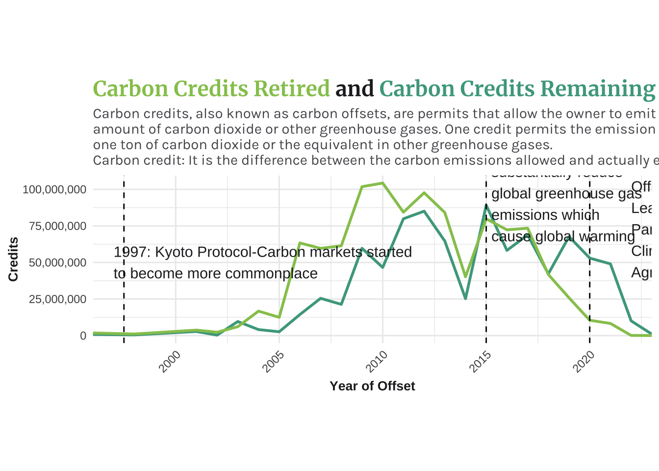
Carbon Credits Remaining versus Carbon Credits Initially Assigned

This graph is suppose to show the general trend of how Credits Retired and Credits Remaining has changed over time. The Kyoto Protocol in 1997 was the first time that international participation in carbon markets started to become more commonplace. A carbon credit is retired once its benefit has taken place. That means it has been used and the carbon benefit it represents has been claimed by the entity that bought it. We see that there is a bigger proportion of Carbon Credits Retired than Credits Remaining Unused. Meaning the Carbon Credits are working as usual.

Code

##~~~~~~~~~~~~~~~~~~~~~~~~~~~~~~~~~~~~~~~~~~~~~~~~~~~~~~~~~~~~~~~~~~~~~~~~~~~~~~
##                    line plot of credits remaining                        ----
##~~~~~~~~~~~~~~~~~~~~~~~~~~~~~~~~~~~~~~~~~~~~~~~~~~~~~~~~~~~~~~~~~~~~~~~~~~~~~~
credits_plot <- carbon_offsets_clean %>% 
  group_by(year_of_offset) %>% 
  summarize(credits_retired = sum(total_credits_retired, na.rm = TRUE),
            credits_remaining = sum(total_credits_remaining, na.rm = TRUE))

# Reshape the data for ggplot
credits_plot_long <- tidyr::pivot_longer(credits_plot, 
                                          cols = c(credits_retired, credits_remaining),
                                          names_to = "type", 
                                          values_to = "credits")

ggplot(credits_plot_long, aes(x = year_of_offset, y = credits, color = type)) +
  geom_line(size=1) +
  scale_color_manual(values = c("credits_retired" = "#95C65CFF", "credits_remaining" = "#4BA68C")) +
  scale_y_continuous(labels = scales::comma) +
  theme_minimal() +
  annotate(geom = "text", x = 1997, y = 50000000,
    label = "1997: Kyoto Protocol-Carbon markets started \nto become more commonplace",
    size = 4, color = "#232226", hjust = "inward") +
  annotate(geom = "text", x = 2015.25, y = 90000000,
    label = "2015: Paris Agreement adopted to\nsubstantially reduce\nglobal greenhouse gas\nemissions which\ncause global warming
    ",
    size = 4, color = "#232226", hjust = "left") +
  annotate(geom = "text", x = 2022, y = 80000000,
    label = "2020: U.S.\nOfficialy\nLeaves\nParis\nClimate\nAgreement",
    size = 4, color = "#232226", hjust = "left") +
  geom_vline(xintercept = 1997.5, 
             linetype = "dashed") +
  geom_vline(xintercept = 2020, 
             linetype = "dashed") +
  geom_vline(xintercept = 2015, 
             linetype = "dashed") +
  scale_x_continuous(expand = c(0, 0)) +
  labs(x = "Year of Offset", y = "Credits", color = NULL, 
    title = "<span style='color:#95C65CFF'>Carbon Credits Retired</span> \nand <span style='color:#4BA68C'>Carbon Credits Remaining</span> \nOver Time, 1997 - 2023", 
       subtitle = "Carbon credits, also known as carbon offsets, are permits that allow the owner to emit a certain\namount of carbon dioxide or other greenhouse gases. One credit permits the emission of \none ton of carbon dioxide or the equivalent in other greenhouse gases.\nCarbon credit: It is the difference between the carbon emissions allowed and actually emitted carbon") +
  theme(
    plot.title = element_markdown(color = "#232226", size = 16, face = "bold", family = "merriweather"),
    axis.text.x = element_text(angle = 45, hjust = 1), # Adjust angle and font family here
    legend.position = "none", 
    plot.subtitle = element_text(size = 11, face = "plain", color = "#555459", family = "karla"),
    axis.title.x = element_text(color = "#232226", size = 10, angle = 0, hjust = .5, vjust = 0, face = "bold"),
    axis.title.y = element_text(color = "#232226", size = 10, angle = 90, hjust = .5, vjust = .5, face = "bold"),
    aspect.ratio=3/10)

Credits

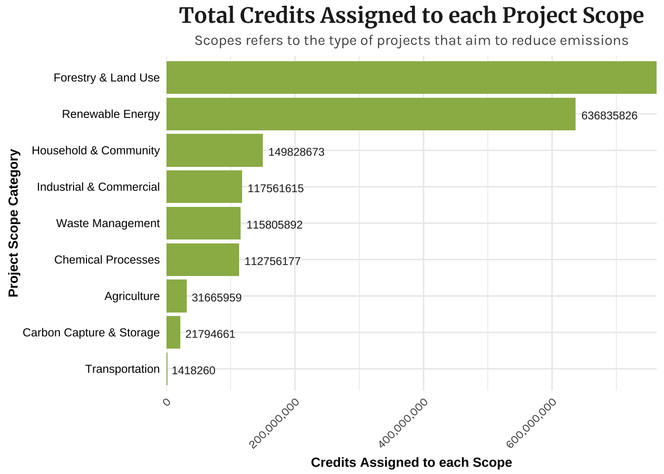
This plot shows all of the scopes (major project categories) and how many carbon credits have been used by each project scope. As shown in the plot Forest & Land Use and Renewable Engery

Code

##~~~~~~~~~~~~~~~~~~~~~~~~~~~~~~~~~~~~~~~~~~~~~~~~~~~~~~~~~~~~~~~~~~~~~~~~~~~~~~
##                          col plot of scopes                         ----
##~~~~~~~~~~~~~~~~~~~~~~~~~~~~~~~~~~~~~~~~~~~~~~~~~~~~~~~~~~~~~~~~~~~~~~~~~~~~~~
scopes <- carbon_offsets_clean %>% 
  mutate(scope = as.factor(scope)) %>% 
  group_by(scope) %>% 
  summarize(total_credits = sum(total_credits_issued, na.rm = TRUE)) %>% 
  filter(total_credits != 0)

scopes_plot <- ggplot(scopes) + 
  #ggalt::geom_lollipop(aes( x = reorder(scope,total_credits),y = total_credits), color = "#9BB655FF", size = 1.5) +
  geom_col(aes( x = reorder(scope,total_credits),y = total_credits), fill = "#9BB655FF", size = 1.5) +
  scale_y_continuous(labels = scales::comma, expand = c(0, 0)) +
  geom_text(aes(x = reorder(scope, total_credits), y = total_credits, label = total_credits),
            vjust = 0.7, color = "#232226", size = 3, hjust = -.1) +  
  theme_minimal() +
  labs(title = "Total Credits Assigned to each Project Scope",
       subtitle = "Scopes refers to the type of projects that aim to reduce emissions", 
       x = "Project Scope Category" ,
       y = "Credits Assigned to each Scope") +
  
  coord_flip() +
  # Annotate custom scale inside plot
  theme(
    plot.title = element_markdown(color = "#232226", size = 16, face = "bold", family = "merriweather", hjust = 0.5),
        axis.text.x = element_text(angle = 45, hjust = 1, family = "karla"), # Adjust angle and font family here
        axis.text.y = element_text(color = "black"),
        legend.position = "none", 
        plot.subtitle = element_text(size = 11, face = "plain", color = "#555459", family = "karla", hjust = 0.5),
        axis.title.x = element_text(color = "black", size = 10, angle = 0, hjust = .5, vjust = 0, face = "bold"),
        axis.title.y = element_text(color = "black", size = 10, angle = 90, hjust = .5, vjust = .5, face = "bold"))

scopes_plot

Code

options(scopes_plot.width =6, scopes_plot.height =3)

Waffle Plot of Credits Issued to Top 7 Countries

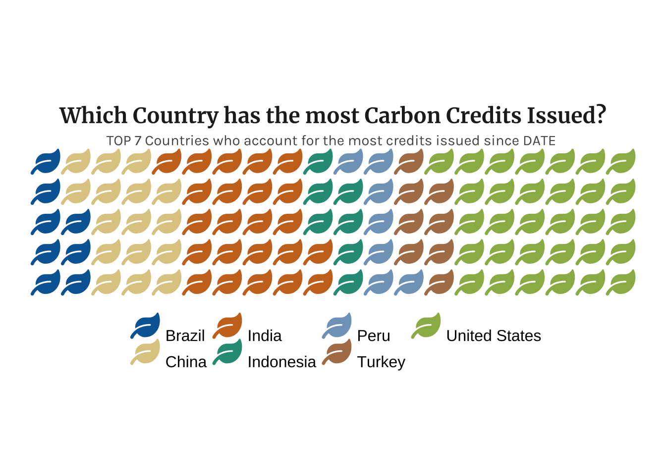
I want to investigate which countries are the ones with most carbon credits assigned.

Code

##~~~~~~~~~~~~~~~~~~~~~~~~~~~~~~~~~~~~~~~~~~~~~~~~~~~~~~~~~~~~~~~~~~~~~~~~~~~~~~
##                    line plot of credits remaining                        ----
##~~~~~~~~~~~~~~~~~~~~~~~~~~~~~~~~~~~~~~~~~~~~~~~~~~~~~~~~~~~~~~~~~~~~~~~~~~~~~~


# subsetted and calcu
carbon_offsets_clean_issued <- carbon_offsets_clean %>%
  group_by(country) %>%
  summarise(total_credits = sum(total_credits_issued, na.rm = TRUE))

top_7_values <- carbon_offsets_clean_issued %>%
  top_n(7, total_credits)

# If you want to keep only the rows with the top 10 values:
filtered_dataframe <- carbon_offsets_clean_issued %>%
  filter(total_credits %in% top_7_values$total_credits)



##~~~~~~~~~~~~~~~~~~~~~~~~~~~~~~~~~~~~~~~~~~~~~~~~~~~~~~~~~~~~~~~~~~~~~~~~~~~~~~
##            waffle plot of credits issued to top 7 countries              ----
##~~~~~~~~~~~~~~~~~~~~~~~~~~~~~~~~~~~~~~~~~~~~~~~~~~~~~~~~~~~~~~~~~~~~~~~~~~~~~~

ggplot(filtered_dataframe, aes(label = country, values = total_credits)) +
  geom_pictogram(n_rows = 5, aes(colour = country), make_proportional = TRUE, family = "fa-solid", size = 7) +
  coord_equal() +
  # paletteer::scale_fill_paletteer_d("rcartocolor::Earth") +
  labs(title = "Which Country has the most Carbon Credits Issued?",
       subtitle = "TOP 7 Countries who account for the most credits issued since DATE ",
       ) +
  scale_color_manual(
    name = NULL, 
    values = c("#0067A2", "#DFCB91", "#CB7223", "#289A84", "#7FA4C2", "#AF7E56", "#9BB655FF"),
    labels = c("Brazil", "China", "India", "Indonesia", "Peru", "Turkey", "United States")) +
  scale_label_pictogram(
    name = NULL,
    values = "leaf",
labels = c("Brazil", "China", "India", "Indonesia", "Peru", "Turkey", "United States")) +  theme_enhance_waffle() +
  theme_void() +
  theme(
    plot.title = element_markdown(color = "#232226", size = 16, face = "bold", family = "merriweather", hjust = 0.5 ),
    plot.subtitle = element_text(size = 11, face = "plain", color = "#555459", family = "karla", hjust = 0.5, margin(t = 5, r = 1, b = 5, l = , unit = "cm")),

    legend.text = element_text(size = 12),
    legend.position = "bottom"
  )

Infographic

Please look at a better Resolution Photo on my Github Repo : How are Carbon Credits Distributed Infographic